The Mathematical Continuum

David Baños Abril

11 de July de 2026 14 min read

Cantorian sets aimed to study the properties of numerical domains as totalities. Before Cantor, establishing the foundations of arithmetic had been a difficult task, particularly regarding irrational quantities and the phenomenon of the continuum. In this article, we will examine the properties of real numbers that were revealed through the use of the concepts of set and cardinality.

On the Mathematical Continuum

Cardinality of the Rational Numbers

Our task in this article will be to apply the concepts of cardinality and transfinite numbers to numerical sets. We will begin with the rational numbers, namely the cardinality of the set $\mathbb{Q}$. Recall that, although the set of rational numbers is dense (given any two rational numbers, there is always another rational number between them distinct from both), it is not continuous. The existence of irrational numbers such as $\sqrt{2}$ or $\pi$ shows that there are gaps that do not correspond to rational numbers.

Under the usual ordering, $\mathbb{Q}$ has no first element because it is not bounded below. Moreover, because of its density, no rational number has an immediate successor. Consider, for example, the interval between $\frac{1}{2}$ and $1$. It makes little sense to ask which number comes immediately after $\frac{1}{2}$. Despite this, the positive rational numbers can be well-ordered by following an arrangement such as the one shown in the image.

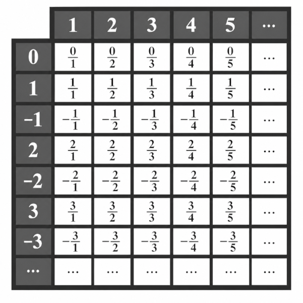
Such an ordering would produce an obviously infinite sequence in which every possible rational number would certainly appear. Since each rational number can be indexed by a natural number (that is, since a bijection can be established), we may state, once again in a counterintuitive way, that the cardinality of the rational numbers is the same as that of the natural numbers, namely, $\left[ \mathbb{Q} \right] = \aleph_{0}$.

The Continuum and the Real Numbers

Cantor initially believed that, just as with the rational numbers, it was possible to establish a bijection between the natural numbers and the real numbers $\mathbb{R}$ (rational and irrational numbers), meaning that both sets would have the same cardinality. The discovery that this was not the case is one of the greatest achievements of Cantor’s set theory.

The Continuous Line

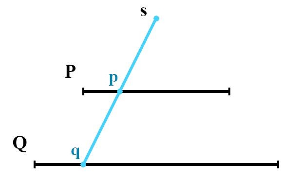
The real number line is also known as the continuous line because it contains no discontinuities. If we define a line, as is often done at school, as a totality of infinitely many points, and knowing that different infinite cardinalities exist, we may ask: How many points are there on a straight line? What is the cardinality of the set of real numbers? As we demonstrate in the image below, the answer is independent of the length of the line. It may seem far from obvious, but every line segment contains the same “number” of infinitely many points.

For every point $q$ on line $Q$ that reaches s, there is an intersection point $p$ on line $P$. Using this construction, we can state that both segments contain the same number of real numbers, regardless of their length.

Defining the Real Numbers

Before considering the cardinality of the real numbers, it will be useful to establish a precise definition of the nature of this numerical domain. At the end of the nineteenth century, this was by no means an easy task: although irrational numbers arise constantly in geometry, defining them solely through arithmetical principles is considerably more difficult. If the rational numbers have been defined from the integers, the central idea is to begin with the rationals in order to characterize the properties of the continuum. We will examine two fundamental contemporary constructions: Dedekind cuts, introduced by the German mathematician Richard Dedekind, with whom Cantor maintained a close relationship, and the definition developed by Cantor himself.

Dedekind Cuts

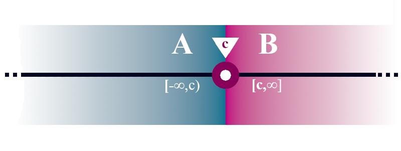
We already know that the rational number line contains gaps: there are positions that correspond to no rational number. These “gaps” are the irrational numbers. We will use this image to understand the concept of a cut (Schnitt), introduced by the German mathematician Richard Dedekind in the late nineteenth century.

The idea of a cut is simple: it consists in dividing the set of rational numbers $\mathbb{Q}$ into two classes $A$ and $B$, such that every element of $A$ is less than every element of $B$. In addition, $A$ must satisfy two important properties. First, if a rational number $a$ belongs to $A$, then every rational number smaller than $a$ also belongs to $A$. In this sense, $A$ extends indefinitely toward the lower end of the rational number line. Second, $A$ has no greatest element: for every rational number $a$ belonging to $A$, there is another rational number $a’$, also belonging to $A$, such that $a \lt a’$. When a partition of this kind is not determined by any rational number, Dedekind takes it as the definition of a new irrational number.

If the cut is produced by a rational number $c$, its two classes can be described as follows:

Subset $A$: all rational numbers less than $c$:
$$A = \left\{ a \in \mathbb{Q}: a \lt c \right\}$$

Subset $B$: all rational numbers greater than or equal to $c$:
$$B = \left\{ b \in \mathbb{Q}: b \geqslant c \right\}$$

In this case, the number $c$ belongs to the second set: it is the least element of $B$. It is also clear that every number $a$ in subset $A$ is less than every number $b$ in subset $B$. If, by contrast, the cut is not produced by any rational number, then there is no rational element occupying the exact boundary between $A$ and $B$. That boundary is precisely the new irrational number defined by the cut.

A number c determines a cut that divides the rational number line into two subsets, $A$ and $B$. These sets have no elements in common. If $c$ is rational, it belongs to subset $B$ as its least element.

Defining the Real Numbers

We can use a cut to define any number $c$. Each cut corresponds to a number, and vice versa. When the number to be defined is rational, it is the least element of set $B$, or equivalently, the least upper bound of $A$, although it does not itself belong to $A$.

But cuts allow us to go further and define irrational numbers as well. Since the subsets consist exclusively of rational numbers, the irrational number is not an element of either $A$ or $B$, but rather the number that Dedekind introduces as corresponding to that cut. Each irrational number corresponds to a unique partition of the rational numbers, and is therefore completely determined by the cut.

Since either subset determines the other, it is normally sufficient to specify the cut by means of the first set $A$, which contains infinitely many elements. Thus, the irrational number $\sqrt{2}$ is defined as the set $A$ such that:

$$A={a \in \mathbb{Q}: a\lt0 \lor a^2\lt2}$$

This definition may seem nonconstructive because it does not provide a finite decimal expression for the number, but it does supply an exact criterion for deciding which rational numbers do or do not belong to the cut. As we will see later, defining the real numbers in terms of subsets of the rationals will prove extremely useful.

Cantor’s Definition of the Real Numbers

Cantor’s definition makes use of what are known as Cauchy sequences, studied by the French mathematician Augustin-Louis Cauchy several decades before Cantor’s investigations. These are sequences of rational numbers whose terms eventually become arbitrarily close to one another. For example, in the following infinite sequence, the terms provide increasingly precise rational approximations:

$$3,\: 3.1,\: 3.14,\: 3.141,\: 3.1415,\: 3.14159,\: \cdots$$

This sequence consists entirely of rational numbers. We need not yet assume the existence of a real number called $\pi$ as the limit of the sequence; what matters for now is that the terms of the sequence draw ever closer to one another. Beyond a certain point, they all lie as close to one another as we please.

Sequences of Rational Numbers

A sequence of rational numbers has as many terms as there are natural numbers. We may therefore understand it as a mathematical function that assigns to each natural number $n$ a rational number $q_n$:

$$s:\mathbb{N}\to\mathbb{Q}, \qquad s(n)=q_n$$

The sequence can then be written as follows:

$$q_1,\: q_2,\: q_3,\: q_4,\: \cdots,\: q_n,\: \cdots$$

The fundamental property of a Cauchy sequence is the following: given any positive rational number $\varepsilon$, there exists an index $N$ such that, beyond that point, the distance between any two subsequent terms is less than $\varepsilon$. That is, for all indices $m,n \geq N$, the following holds:

$$\left|q_m-q_n\right| \lt \varepsilon$$

This condition does not merely say that each term is close to the immediately following term. It says something stronger: all sufficiently advanced terms of the sequence are close to one another, even when their indices are far apart.

In the previous example:

$$3,\: 3.1,\: 3.14,\: 3.141,\: 3.1415,\: 3.14159,\: \cdots$$

if we take, for example, $\varepsilon = 0.001$, we see that, beyond a certain index, all terms of the sequence differ from one another by less than $0.001$. The same will occur for any positive value of $\varepsilon$, however small we choose it: we need only proceed far enough along the sequence.

Cauchy Sequences and Real Numbers

The decisive idea is that a Cauchy sequence of rational numbers need not determine any rational number. Its terms may become indefinitely close to one another without there being a rational number that occupies exactly the position toward which the sequence points. In such cases, Cantor interprets the sequence as determining a new number: a real number.

Thus, rather than taking the real numbers as something already given, Cantor shows how they can be constructed from sequences of rational numbers. Some of these sequences determine rational numbers; others determine irrational numbers. In both cases, however, the real number is fixed by the internal behavior of the sequence.

It is important, however, to emphasize one qualification: the same real quantity can be represented by many different rational sequences. For example, two different sequences may “point” to the same number and approach one another until they become indistinguishable from the perspective of the Cauchy condition. We therefore do not identify each real number with a single sequence, but with an equivalence class of Cauchy sequences. We may then say that the points of the continuum are determined by equivalence classes of Cauchy sequences of rational numbers. This is Cantor’s method for defining the real numbers from the rationals without presupposing the existence of the continuum.

Subsets of Rational Numbers

We have seen, by two different routes, that the real numbers can be determined from the rational numbers. In Dedekind’s construction, each real number is associated with a cut, that is, with a certain partition of the set $\mathbb{Q}$. In Cantor’s construction, each real number is associated with a class of Cauchy sequences of rational numbers. In both cases, the continuum is not introduced as a primitive geometric intuition, but through arithmetical constructions carried out over the domain of the rational numbers.

This observation allows us to connect the definition of the real numbers with set theory. Both Dedekind and Cantor show that a point on the continuous line is determined from an infinite totality of rational numbers. Not every infinite set of rational numbers, however, determines a point on the real number line. The natural numbers, for example, form an infinite set of rational numbers, but they do not identify any particular position on the continuum. For the correspondence to work, those rational numbers must be organized in a precise way: as the left-hand portion of a boundary in Dedekind’s construction, or as a sequence of increasingly tight approximations in Cantor’s.

Infinite Strings of 0s and 1s

Dedekind’s and Cantor’s definitions lead us to the same idea: a real number can be determined by an infinite totality of rational numbers organized in a precise way. To study its cardinality, however, it is useful to represent this information in the simplest possible form. One way to do this is to translate each of these rational totalities into an infinite string of $0$s and $1$s.

Consider first a Dedekind cut. Since the rational numbers can be enumerated, as we saw in the first section of this article, we may write them as a sequence:

$$q_1,\ q_2,\ q_3,\ q_4,\ \cdots$$

A cut selects some of these rational numbers: those lying on the left-hand side of the boundary. We can then move through the preceding enumeration and write a $1$ whenever the rational number $q_n$ belongs to that left-hand portion, and a $0$ whenever it does not. In this way, the cut is encoded by an infinite string:

$$1,\ 1,\ 0,\ 1,\ 0,\ 0,\ 1,\ \cdots$$

The same idea can be applied to Cantor’s definition. A sequence of rational numbers contains a countable number of terms. If we fix a way of enumerating the rational numbers, we can also record which rational numbers occur in a given approximation.

Now, an infinite string of $0$s and $1$s is exactly what we need to describe a subset of a countable set. If we enumerate the rational numbers as $q_1,q_2,q_3,\ldots$, each binary string determines a subset of $\mathbb{Q}$: the subset consisting of those $q_n$ whose position contains a $1$. Conversely, each subset of $\mathbb{Q}$ determines an infinite binary string. Thus, from the standpoint of cardinality, speaking of infinite configurations of rational numbers is equivalent to speaking of infinite strings of $0$s and $1$s. Since there are two possible choices at each of the $\aleph_0$ positions in the string, the total number of such strings is:

$$2^{\aleph_0}$$

This reveals the deep connection between the continuum and the power set of the rational numbers. The real numbers do not arise from every arbitrary subset of $\mathbb{Q}$, but from rational configurations possessing a particular structure. Yet all such configurations lie within the broader space of infinite binary strings, that is, within the set of all possible selections of rational numbers. The cardinality of the continuum (usually denoted by $\mathfrak{c}$) is therefore tied to this power:

$$\left[\mathbb{R}\right]=\mathfrak{c}=2^{\aleph_0}$$

Diagonal Proof

That the infinity of the real numbers is greater than that of the natural numbers can be proved by using the diagonal argument introduced in the previous article. If the number of real numbers were equal to the number of natural numbers, we could index every real number by a natural number and construct a two-dimensional table.

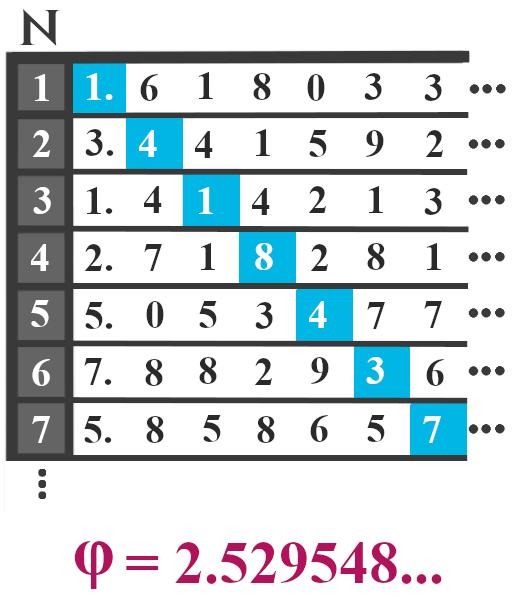
But for any such table, we can generate a number $\varphi$ that is real yet does not appear in the table. This number will differ from every number in the table in at least one digit.

The Continuum Hypothesis

In the previous article, we saw that Cantor’s Theorem guarantees the existence of a cardinal greater than $\aleph_0$. Given a countable set such as $\mathbb{N}$, its power set necessarily has a greater cardinality:

$$\aleph_0 \lt 2^{\aleph_0}$$

We can now understand more clearly what this new cardinal represents. It is not merely an abstract cardinal arising from the power set, but the cardinality of the continuum: the number of points on a line, or equivalently, the number of real numbers.

$$\left[\mathbb{R}\right]=\mathfrak{c}=2^{\aleph_0}$$

As we have already anticipated, the decisive question is whether this new infinity is the first cardinal after $\aleph_0$. Put differently: we know that the continuum has a greater cardinality than the natural numbers, but is there an intermediate cardinal between the cardinality of the natural numbers and that of the continuous line? Cantor conjectured that there was not. According to his Continuum Hypothesis, every infinite subset of the real number line must have either the cardinality of the natural numbers or the cardinality of the continuum. There would be no third, intermediate possibility. In modern notation, this is expressed by saying that the cardinality of the continuum coincides with the first transfinite cardinal after $\aleph_0$:

$$\mathfrak{c}=\aleph_1$$

This question would profoundly shape the subsequent development of set theory. Long after Cantor, the work of Gödel and Cohen showed that the Continuum Hypothesis cannot be settled from the usual axioms of set theory: neither it nor its negation follows from them, provided those axioms are consistent. But that story belongs to a later stage of Cantor’s paradise.

Cardinality of the Rational Numbers

The Continuum and the Real Numbers

The Continuous Line

Defining the Real Numbers

Dedekind Cuts

Defining the Real Numbers

Cantor’s Definition of the Real Numbers

Sequences of Rational Numbers

Cauchy Sequences and Real Numbers

Subsets of Rational Numbers

Infinite Strings of 0s and 1s

Diagonal Proof

The Continuum Hypothesis

Recommended Reading

Related articles