Cantor’s Set Theory

David Baños Abril

11 de July de 2026 15 min read

The mathematician Georg Cantor was the mind that would, once and for all, succeed in giving the obscure concept of infinity a precise mathematical treatment. To this end, he created the magnificent Set Theory—the tool that would allow him to grapple with the ever-elusive concept of infinity.

Paradoxes of Infinity

By the end of the nineteenth century, Analysis was one of the most powerful mathematical tools and the principal link between pure Mathematics and its applications in the Natural Sciences. Despite having dispensed with controversial concepts such as “infinitesimals,” Analysis was still far from the level of rigor that was beginning to be demanded throughout mathematics. The appearance of the ever-confusing and paradoxical infinite in each new mathematical discovery remained a persistent source of difficulty.

Potential Infinity

We have already seen in the previous article the difficulties associated with mathematical infinity. These problems were enough to make some mathematicians reject infinity and relegate it to philosophical discussion. For many of them, infinity is simply the possibility of continuing a procedure over and over again. This is what Aristotle called potential infinity: infinity as a possibility. For Gauss, what matters is the limit, the point toward which an increasing quantity tends. An example is the sequence $4.4, \, 4.49, \, 4.499, \cdots $, which could continue indefinitely but has $4.5$ as its limit. Some series, known as divergent series, do not converge to a point. Some of them grow without bound; we say that such series have their limit at $\infty$.

Cantor and Infinity

It is one thing for a rational being such as a human to reflect on the possibility of continuing an operation indefinitely, as in counting, and quite another to understand infinity as a closed and bounded object. Treating infinity as actual infinity, that is, as a distinct unity, appears in some sense to violate elementary logic, since it attempts to delimit and specify precisely what is defined as having no limit. Yet we have already seen that evaluating convergent series requires us to regard their endless number of terms as a single whole. Any reduction to a finite number of terms yields only an approximation.

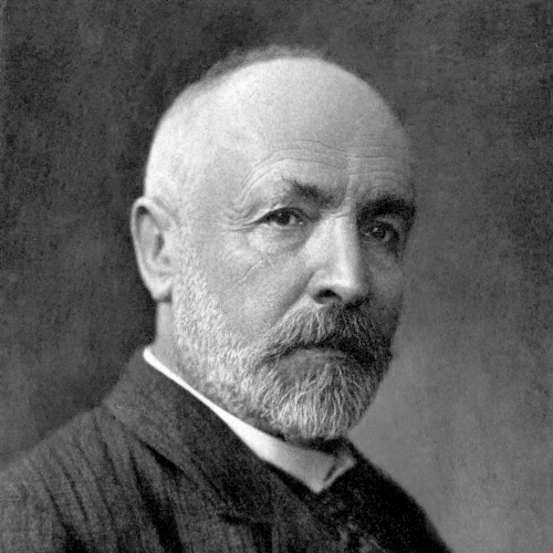
The central figure of this article embraced this latter interpretation of infinity and pursued it to its ultimate consequences. Georg Cantor, born into the German community of Saint Petersburg and possessed of a genius rarely surpassed in the history of mathematics, was simultaneously a mathematician, philosopher, and theologian, and he took pride in drawing from such diverse sources. We owe Set Theory to him, a new branch of mathematics that enabled him to deal conceptually with infinity. We will draw primarily on his 1883 work, “Foundations of a General Theory of Sets.”

Set Theory

The mathematical idea of a set is not very different from the everyday meaning of the word. Cantor understood a set (Menge in the original German) as a collection of definite elements that can be conceived as a unity. A set, therefore, is not merely a list of elements. It is a set when the totality of those elements is itself a unity. Thus, the elements Chico, Groucho, Harpo, and Zeppo form a set: the Marx Brothers. As we shall see, Cantor allowed for sets with infinitely many elements. We denote sets with braces:

Marx Brothers = {Chico, Groucho, Harpo, Zeppo}

Set Theory aims to provide a foundation for all of Arithmetic, supplying the basis from which the natural numbers and the deductions that follow from them can be precisely defined. To do so, it must rely on concepts that are simple and clear, yet powerful enough to support the immense mathematical edifice accumulated over so many centuries. Accordingly, in our exposition we will not even assume the concept of number in advance. Our first step will be to justify the natural numbers from this notion of a set.

Power

To compare sets in terms of their number of elements, Cantor introduced the notion of the set’s power. Two sets are said to have the same power when a bijection can be established between them, meaning that their elements can be paired without leaving any element unmatched.

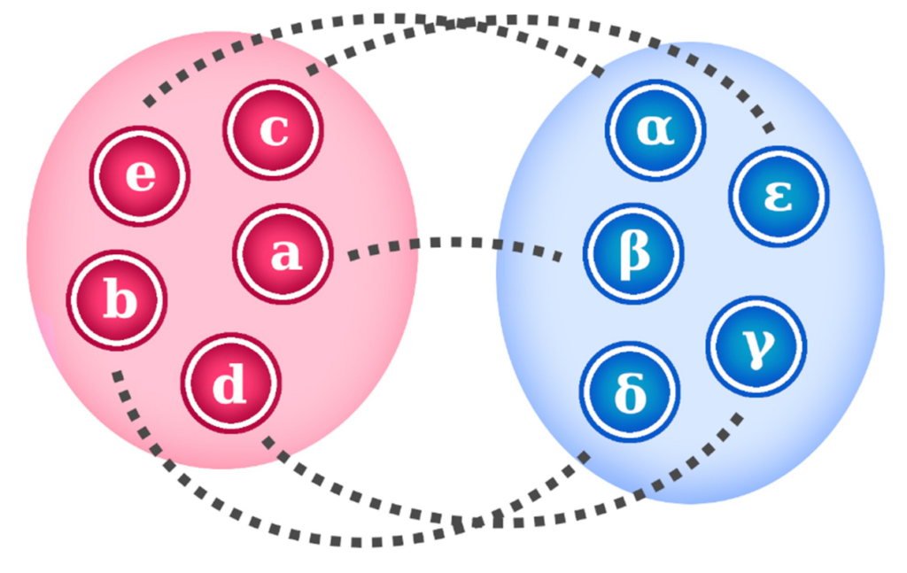
Diagrama de dos conjuntos equipotentes unidos por una biyección — Example of two equipotent sets. As shown, it does not matter which elements are paired with one another. Nor is it assumed that the elements are ordered. As long as pairs can be formed without any element being excluded from the bijection, the sets are equipotent.

Intuitively, the concept of power corresponds to the familiar idea of the number of elements. This may serve as a useful guide, but for the remainder of the article it will be advisable to adhere to the strict mathematical definitions.

Well-Ordered Sets

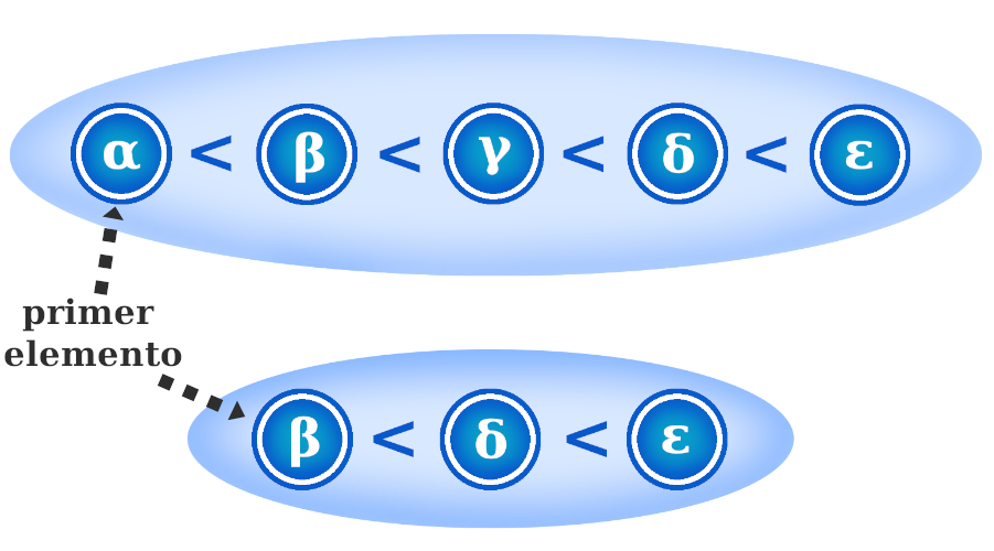
A key concept underpinning Cantor’s entire Set Theory is that of a well-ordered set. A set is well ordered if it has an initial or first element. We define an initial element as an element $n$ such that, for every element $m$ of the set, $n \preceq m$; that is, $n$ precedes $m$. We use “precedes” so as not to restrict ourselves to numerical sets whose elements can be related as less than or greater than one another. To complete the definition of a well order, this first-element condition must hold for every possible subset: each subset must have an initial element. In other words, two conditions must be satisfied: first, a linear order, which means that any two distinct elements of the set must always be related by one coming after the other; and second, the first-element condition just described for every subset.

In Cantor’s work, “well ordered” came close to being synonymous with “set.” If a collection of elements can be well ordered, then it is a set, and conversely. This identification between sethood and the possibility of well ordering belongs to Cantor’s historical context. In modern set theory, however, a set is not defined by being well ordered or well-orderable: a well order is an additional structure. The statement that every set can be well ordered is a consequence of the Axiom of Choice, not part of the definition of a set itself. We will return to this in later chapters. For now, however, we will retain a historical perspective on the problem.

Diagrama de Conjuntos Bien Ordenados — *At the top of this example we see a finite well-ordered set. All its possible subsets, such as the example below, have a first element, as required by the definition of a well order.*

Well-Ordered Numbers

The natural numbers are an example of a linearly well-ordered set:

\mathbb{N} = \left\{ 1, 2, 3, 4, \cdots \right\}

A subset of the natural numbers such as $\left\{ 1456, 45, 679, 13946695 \right\}$ can be well ordered:

$$45 < 679 < 1456 < 13946695$$

Consider the integers $\mathbb{Z}$ ordered as follows:

$$ \mathbb{Z} = \left\{ \cdots -3,-2,-1,0,1,2,3\cdots \right\}$$

This order is linear, since any two distinct elements can be placed in a relation of succession. It is not, however, a well order, because there is no least initial element.

Set Theory and Numbers

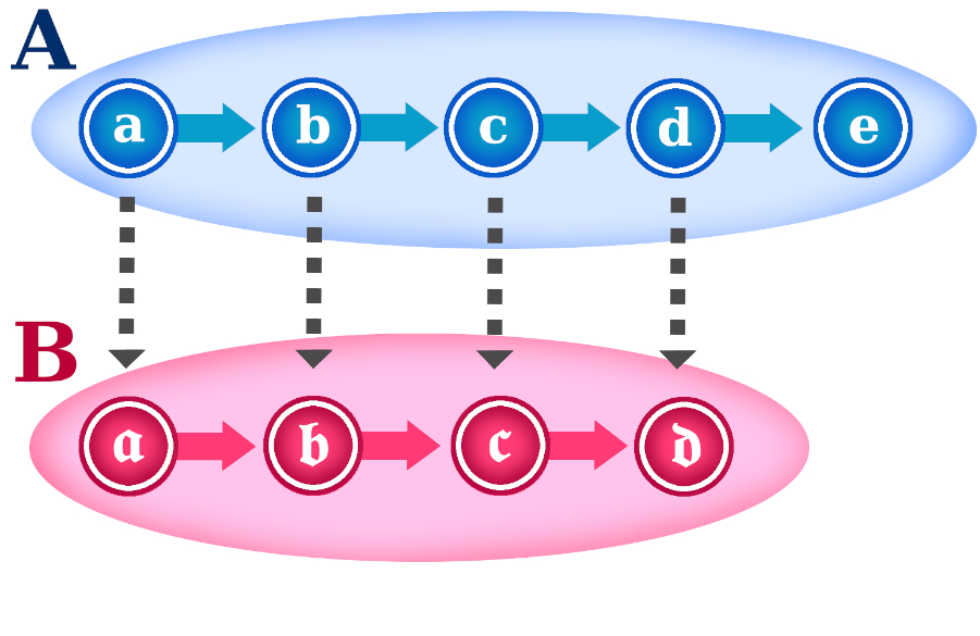
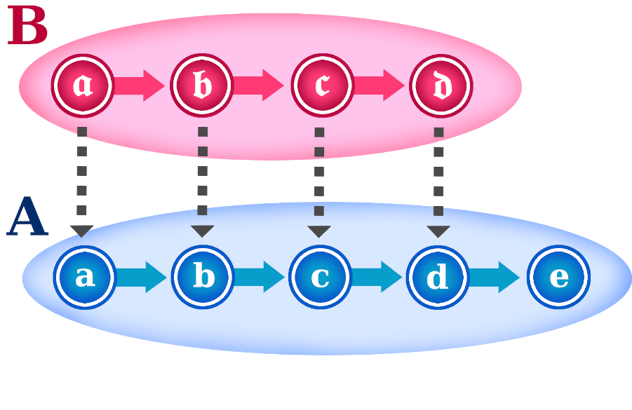
We call an enumeration (or counting, Anzahl in German) a mapping in which, whenever two elements occur successively in one set, their corresponding elements also occur successively in the other, and the enumerating set covers every element of the set being enumerated. A well-ordered set has an enumeration. Any sets that can enumerate one another share the same order type.

Diagrama de un conjunto A enumerando un conjunto B

Diagrama de un conjunto B que no puede enumerar un conjunto A — *The upper image shows an enumeration from set* $A$ *to set* $B$*. We say that* $A$ *enumerates* $B$*. In the lower image, however, we see that* $B$ *does not enumerate* $A$*, because it does not reach all of its elements. Cantor abstracts this fact and states that these sets have different order types, and that the order type of* $A$ *is greater than that of* $B$.

Ordinal Numbers

If a set of order type $\alpha$ enumerates another of order type $\beta$, but not conversely, then they clearly have different order types. Moreover, these two order types are themselves well ordered: $\alpha$ is greater than $\beta$, or, more formally, $\beta$ is the order type of only an initial segment of $\alpha$. Two conclusions follow. In Set Theory, Cantor grounds numbers in these order types. The well-ordered sequence of order types is what Cantor calls ordinal numbers, or simply numbers.

The first conclusion is that every well-ordered set has an order type, that is, an associated ordinal number. Moreover, these order types do not occur in isolation: they can be compared and arranged in an ordered sequence. Thus, from a given ordinal we can consider its successor, and then the successor of that successor, forming a series:

$$\alpha,\ \alpha^{\prime},\ \alpha^{\prime\prime},\ \alpha^{\prime\prime\prime},\ \cdots$$

In the most familiar case, this sequence corresponds to the order of the natural numbers:

$$1,\ 2,\ 3,\ 4,\ \cdots$$

We will use this ordinal sequence as a reference scale, or as an enumerator, to describe the order type of other well-ordered sets.

Power and Order in Set Theory

We have imposed the condition that the counting of sets must follow a linear order. As our everyday experience makes clear, the result of that counting does not change if we count in a different order. But this is because we are dealing with finite sets.

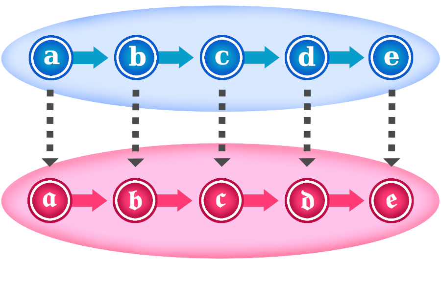
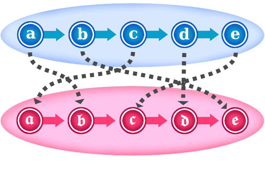
Diagrama de una biyección equivalente a una enumeración entre conjuntos A y B.

Diagrama de una biyección que no es equivalente a una enumeración entre conjuntos A y B. — This diagram shows two different bijections. In both, no element is left unmatched, so the blue and pink sets are equipotent. Only the upper mapping, however, is an enumeration, which is what allows us to determine the set’s ordinal. *Because these are finite sets, their power and ordinal coincide*.

For infinite sets, we will now see that different enumerations can produce different ordinal numbers for the same set, depending on how its elements are ordered. It is therefore necessary to distinguish between the number of elements in a set (its power or cardinality) and its ordinal (or order type). This distinction must be kept clear, since Cantor’s early work is founded upon it.

Set Theory and Transfinite Ordinals

The Infinite Ordinal

The sequences $ a_1, a_2, a_3, \cdots $ and $ a_7, a_8, a_9, \cdots $ can both be enumerated by the infinitely many natural numbers. Which ordinal corresponds to a sequence of this kind? Just as mathematics uses $n$ (or the nth term) to denote an arbitrary natural number, Cantor conceived the ordinal number $\omega$ as the ordinal that follows all finite ordinals: an order type expressing an infinite sequence given as a completed whole. Thus, both example sets have ordinal $\omega$, the infinite ordinal. Cantor thereby fulfilled his aim of establishing infinity as a delimited and defined object.

We must emphasize that $\omega$ is not the totality of all numbers; it is the ordinal number that enumerates the complete sequence of finite integers. As an advocate of actual infinity, Cantor replaced the symbol $\infty$ with $\omega$ precisely to avoid a potential-infinity interpretation.

Transfinite Ordinals

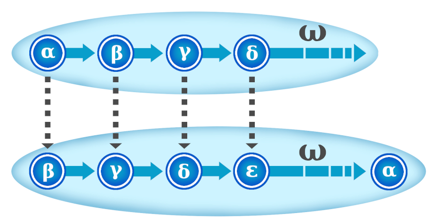
Now consider the sequences $ a_1, a_2, a_3, \cdots$ and $ b_2, b_3, \cdots, b_1$. Both have the same number of elements: the power of the natural numbers. The first also has ordinal $\omega$. The second set, however, has an initial part of order $\omega$, followed by one additional element, $b_1$. This final element lies beyond the infinite enumeration of $\omega$, which never reaches it.

Therefore, a set of order $\omega$ cannot enumerate another set whose order type is greater than $\omega$. We consequently say that the latter set has ordinal $\omega + 1$. Thus, unlike the case of finite sets, the ordinal of an infinite set depends on how its elements are ordered. For example, $ a_2, a_3, \cdots, a_1 $ and $ a_3, \cdots, a_1, a_2 $ contain the same elements and clearly have the same power, but they are ordered differently and therefore form sets with different ordinals: $\omega + 1$ and $\omega + 2$, respectively.

Diagrama que muestra dos conjuntos , uno de ordinal omega y otro de ordinal omega + 1 — Although they contain the same infinite set of elements, the upper set cannot enumerate the lower one, because the latter has an order type greater than $\omega$.

The First Principle of Generation

It is always possible to add one to a given number. Cantor called this the First Principle of Generation, and it accounts for the infinitely many natural numbers. As we can see, however, it also applies to the ordinal $\omega$, so the series continues with $\omega + 1$, $\omega + 2$, $\omega + 3$, and so on.

All these numbers are known as transfinite ordinals. These transfinite numbers are themselves ordered from least to greatest (with $\omega$ as the smallest of them), and we can therefore define arithmetic operations on them, justifying their treatment as numbers. Yet they have properties that seem “strange” when compared with the natural numbers. Adding the infinite ordinal $\omega$ to $1$ yields $\omega$; the initial unit has no effect on the infinite order. But if we regard the infinite ordered sequence as an object given in its complete and determinate form, then adding $1$ after $\omega$ produces an entirely different number: $\omega + 1$. The commutative property therefore fails:

$$1+ \omega \neq \omega +1$$

The Second Principle of Generation

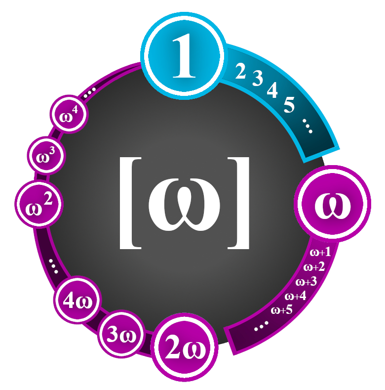
Cantor proposed a Second Principle of Generation: to establish a limit ordinal toward which an infinite sequence tends, defined as a number greater than every member of that sequence. In the case of the sequence of natural numbers, its limit is, as we have seen, the ordinal $\omega$. For the sequence $\omega + 1$, $\omega + 2$, $\omega + 3$, and so on, the limit ordinal is $\omega + \omega$, or equivalently $2\omega$ (in later texts, Cantor would write $\omega \cdot 2$). An example of a set with ordinal $2\omega$ is the sequence of all even numbers followed by all odd numbers:

$$\prec 2 \prec 4 \prec 6 \prec \cdots \prec 1 \prec 3 \prec 5 \prec 7 \prec \cdots \omega $$

This new principle of establishing infinite limits can be continued again and again: $2\omega + 1$, $2\omega + 2$, $2\omega + 3$, and so on; then $2\omega + \omega = 3\omega$, followed by $4\omega$, $5\omega$, $6\omega$, and so forth; then $\omega\omega = \omega^2$, followed by $\omega^3$, $\omega^4$, and ultimately $\omega^\omega$.

Matriz bisimensional para mostrar la enumeración de ordinales transfinitos. — Example of a two-dimensional matrix of $\omega^2$. We may imagine dimensions higher than two as corresponding to transfinite ordinals such as $\omega^3$, $\omega^4$, $\omega^5$, and so on, including even an infinite-dimensional matrix in the case of $\omega^\omega$.

The Second Principle of Generation may appear insufficiently justified. Cantor initially made no effort to prove these principles, although he acknowledged that they were a logical consequence of treating infinity as actual. Later discoveries would provide support for these assumptions.

The Third Principle

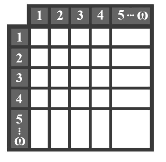
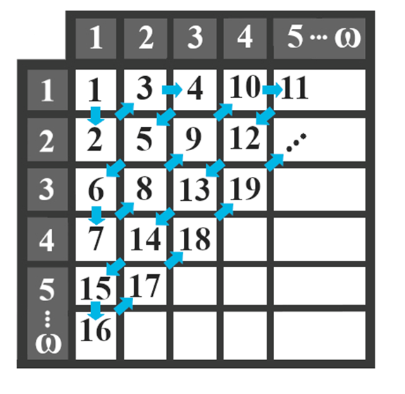
It may seem that this sequence merely leads us into an immeasurable progression of monstrous transfinite quantities. Cantor’s work would have little to offer if it ended there. Set Theory, however, still has much more to reveal. Cantor established a third principle, the Principle of Limitation: all the transfinite ordinals considered so far are equipotent with the set of natural numbers; in other words, they designate sets containing the same number of elements. We have seen this in the case of a set of order $2\omega$, formed by the infinite sequence of even numbers followed by the infinite sequence of odd numbers. Although it is “doubly infinite,” it still contains “only” as many elements as the set of natural numbers.

The matrix of $\omega^2$ can be completely covered by the set of natural numbers. No cell is left uncovered if a diagonal path is followed through the matrix. This demonstrates that a bijection can be established between the set of natural numbers and a set of ordinal $\omega^2$, and therefore that both sets have the same power.

A diagram summarizing the transfinite ordinals discussed so far. Beginning with unity, the infinitely many natural numbers (in blue) $1, 2, 3, 4, \cdots$ arise through the Principle of Addition. Then, through the Second Principle of Generation, this entire completed sequence is treated as a new mathematical object, denoted by $\omega$, to which the first principle can again be applied, producing the series $\omega$, $\omega + 1$, $\omega + 2$, $\omega + 3 \cdots$. We define the transfinite ordinals (in violet) as all the numbers generated by these two principles. By the third principle, or Principle of Limitation, they all have the same power: the power of the natural numbers $\left[ \omega \right]$.

Beyond the Natural Numbers

Although the set of natural numbers can be assigned infinitely many order types, there is clearly one and only one that is the smallest of all: $\omega$. Every countably infinite set admits a well order of type $\omega$, which is the least possible ordinal for a countably infinite totality. We say that all sets that can be placed in bijection with one another share the same power, or, as Cantor would call it in later texts, the same cardinal number.

The next question is evident: are there sets with infinitely many elements whose power is greater than that of the natural numbers? The answer is yes, and this will be the subject of our next article.